On word embeddings - Part 1
Word embeddings popularized by word2vec are pervasive in current NLP applications. The history of word embeddings, however, goes back a lot further. This post explores the history of word embeddings in the context of language modelling.
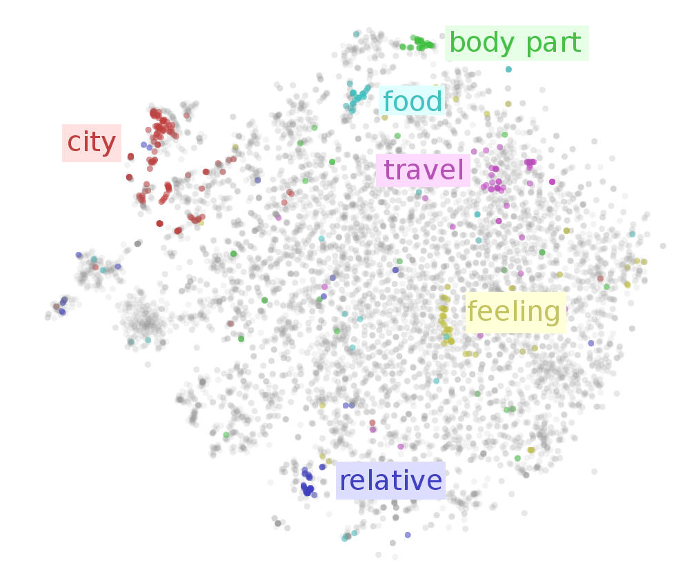
This post presents the most well-known models for learning word embeddings based on language modelling.
Table of contents:
Unsupervisedly learned word embeddings have been exceptionally successful in many NLP tasks and are frequently seen as something akin to a silver bullet. In fact, in many NLP architectures, they have almost completely replaced traditional distributional features such as Brown clusters and LSA features.
Proceedings of last year's ACL and EMNLP conferences have been dominated by word embeddings, with some people musing that Embedding Methods in Natural Language Processing was a more fitting name for EMNLP. This year's ACL features not one but two workshops on word embeddings.
Semantic relations between word embeddings seem nothing short of magical to the uninitiated and Deep Learning NLP talks frequently prelude with the notorious \(king - man + woman \approx queen \) slide, while a recent article in Communications of the ACM hails word embeddings as the primary reason for NLP's breakout.
This post will be the first in a series that aims to give an extensive overview of word embeddings showcasing why this hype may or may not be warranted. In the course of this review, we will try to connect the disperse literature on word embedding models, highlighting many models, applications and interesting features of word embeddings, with a focus on multilingual embedding models and word embedding evaluation tasks in later posts.
This first post lays the foundations by presenting current word embeddings based on language modelling. While many of these models have been discussed at length, we hope that investigating and discussing their merits in the context of past and current research will provide new insights.
A brief note on nomenclature: In the following we will use the currently prevalent term word embeddings to refer to dense representations of words in a low-dimensional vector space. Interchangeable terms are word vectors and distributed representations. We will particularly focus on neural word embeddings, i.e. word embeddings learned by a neural network.
A brief history of word embeddings
Since the 1990s, vector space models have been used in distributional semantics. During this time, many models for estimating continuous representations of words have been developed, including Latent Semantic Analysis (LSA) and Latent Dirichlet Allocation (LDA). Have a look at this blog post for a more detailed overview of distributional semantics history in the context of word embeddings.
Bengio et al. refer to word embeddings as distributed representations of words in 2003 and train them in a neural language model jointly with the model's parameters. First to show the utility of pre-trained word embeddings were arguably Collobert and Weston in 2008. Their landmark paper A unified architecture for natural language processing not only establishes word embeddings as a useful tool for downstream tasks, but also introduces a neural network architecture that forms the foundation for many current approaches. However, the eventual popularization of word embeddings can be attributed to Mikolov et al. in 2013 who created word2vec, a toolkit that allows the seamless training and use of pre-trained embeddings. In 2014, Pennington et al. released GloVe, a competitive set of pre-trained word embeddings, signalling that word embeddings had reached the main stream.
Word embeddings are one of the few currently successful applications of unsupervised learning. Their main benefit arguably is that they don't require expensive annotation, but can be derived from large unannotated corpora that are readily available. Pre-trained embeddings can then be used in downstream tasks that use small amounts of labeled data.
Word embedding models
Naturally, every feed-forward neural network that takes words from a vocabulary as input and embeds them as vectors into a lower dimensional space, which it then fine-tunes through back-propagation, necessarily yields word embeddings as the weights of the first layer, which is usually referred to as Embedding Layer.
The main difference between such a network that produces word embeddings as a by-product and a method such as word2vec whose explicit goal is the generation of word embeddings is its computational complexity. Generating word embeddings with a very deep architecture is simply too computationally expensive for a large vocabulary. This is the main reason why it took until 2013 for word embeddings to explode onto the NLP stage; computational complexity is a key trade-off for word embedding models and will be a recurring theme in our review.
Another difference is the training objective: word2vec and GloVe are geared towards producing word embeddings that encode general semantic relationships, which are beneficial to many downstream tasks; notably, word embeddings trained this way won't be helpful in tasks that do not rely on these kind of relationships. In contrast, regular neural networks typically produce task-specific embeddings that are only of limited use elsewhere. Note that a task that relies on semantically coherent representations such as language modelling will produce similar embeddings to word embedding models, which we will investigate in the next chapter.
As a side-note, word2vec and Glove might be said to be to NLP what VGGNet is to vision, i.e. a common weight initialisation that provides generally helpful features without the need for lengthy training.
To facilitate comparison between models, we assume the following notational standards: We assume a training corpus containing a sequence of \(T\) training words \(w_1, w_2, w_3, \cdots, w_T\) that belong to a vocabulary \(V\) whose size is \(|V|\). Our models generally consider a context of \( n \) words. We associate every word with an input embedding \( v_w \) (the eponymous word embedding in the Embedding Layer) with \(d\) dimensions and an output embedding \( v'_w \) (another word representation whose role will soon become clearer). We finally optimize an objective function \(J_\theta\) with regard to our model parameters \(\theta\) and our model outputs some score \(f_\theta(x)\) for every input \( x \).
A note on language modelling
Word embedding models are quite closely intertwined with language models. The quality of language models is measured based on their ability to learn a probability distribution over words in \( V \). In fact, many state-of-the-art word embedding models try to predict the next word in a sequence to some extent. Additionally, word embedding models are often evaluated using perplexity, a cross-entropy based measure borrowed from language modelling.
Before we get into the gritty details of word embedding models, let us briefly talk about some language modelling fundamentals.
Language models generally try to compute the probability of a word \(w_t\) given its \(n - 1\) previous words, i.e. \(p(w_t \: | \: w_{t-1} , \cdots w_{t-n+1})\). By applying the chain rule together with the Markov assumption, we can approximate the probability of a whole sentence or document by the product of the probabilities of each word given its \(n\) previous words:
\(p(w_1 , \cdots , w_T) = \prod\limits_i p(w_i \: | \: w_{i-1} , \cdots , w_{i-n+1}) \).
In n-gram based language models, we can calculate a word's probability based on the frequencies of its constituent n-grams:
\( p(w_t \: | \: w_{t-1} , \cdots , w_{t-n+1}) = \dfrac{count(w_{t-n+1}, \cdots , w_{t-1},w_t)}{count({w_{t-n+1}, \cdots , w_{t-1}})}\).
Setting \(n = 2\) yields bigram probabilities, while \(n = 5\) together with Kneser-Ney smoothing leads to smoothed 5-gram models that have been found to be a strong baseline for language modelling. For more details, you can refer to these slides from Stanford.
In neural networks, we achieve the same objective using the well-known softmax layer:
\(p(w_t \: | \: w_{t-1} , \cdots , w_{t-n+1}) = \dfrac{\text{exp}({h^\top v'_{w_t}})}{\sum_{w_i \in V} \text{exp}({h^\top v'_{w_i}})} \).
The inner product \( h^\top v'_{w_t} \) computes the (unnormalized) log-probability of word \( w_t \), which we normalize by the sum of the log-probabilities of all words in \( V \). \(h\) is the output vector of the penultimate network layer (the hidden layer in the feed-forward network in Figure 1), while \(v'_w\) is the output embedding of word \(w \), i.e. its representation in the weight matrix of the softmax layer. Note that even though \(v'_w\) represents the word \(w\), it is learned separately from the input word embedding \(v_w\), as the multiplications both vectors are involved in differ (\(v_w\) is multiplied with an index vector, \(v'_w\) with \(h\)).
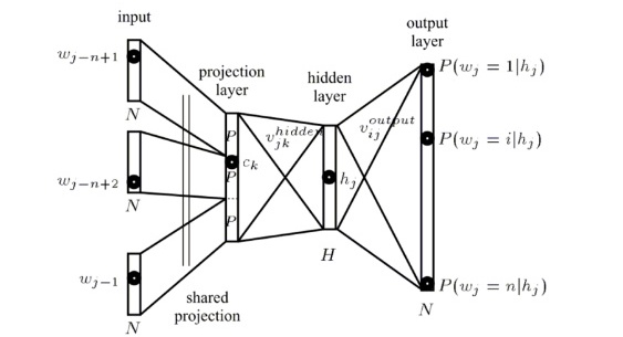
Note that we need to calculate the probability of every word \( w \) at the output layer of the neural network. To do this efficiently, we perform a matrix multiplication between \(h\) and a weight matrix whose rows consist of \(v'_w\) of all words \(w\) in \(V\). We then feed the resulting vector, which is often referred to as a logit, i.e. the output of a previous layer that is not a probability, with \(d = |V|\) into the softmax, while the softmax layer "squashes" the vector to a probability distribution over the words in \(V\).
Note that the softmax layer (in contrast to the previous n-gram calculations) only implicitly takes into account \(n\) previous words: LSTMs, which are typically used for neural language models, encode these in their state \(h\), while Bengio's neural language model, which we will see in the next chapter, feeds the previous \(n\) words through a feed-forward layer.
Keep this softmax layer in mind, as many of the subsequent word embedding models will use it in some fashion.
Using this softmax layer, the model tries to maximize the probability of predicting the correct word at every timestep \( t \). The whole model thus tries to maximize the averaged log probability of the whole corpus:
\(J_\theta = \frac{1}{T} \text{log} \space p(w_1 , \cdots , w_T)\).
Analogously, through application of the chain rule, it is usually trained to maximize the average of the log probabilities of all words in the corpus given their previous \( n \) words:
\(J_\theta = \frac{1}{T}\sum\limits_{t=1}^T\ \text{log} \space p(w_t \: | \: w_{t-1} , \cdots , w_{t-n+1})\).
To sample words from the language model at test time, we can either greedily choose the word with the highest probability \(p(w_t \: | \: w_{t-1} \cdots w_{t-n+1})\) at every time step \( t \) or use beam search. We can do this for instance to generate arbitrary text sequences as in Karpathy's Char-RNN or as part of a sequence prediction task, where an LSTM is used as the decoder.
Classic neural language model
The classic neural language model proposed by Bengio et al. [1] in 2003 consists of a one-hidden layer feed-forward neural network that predicts the next word in a sequence as in Figure 2.
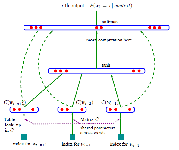
Their model maximizes what we've described above as the prototypical neural language model objective (we omit the regularization term for simplicity):
\(J_\theta = \frac{1}{T}\sum\limits_{t=1}^T\ \text{log} \space f(w_t , w_{t-1} , \cdots , w_{t-n+1})\).
\( f(w_t , w_{t-1} , \cdots , w_{t-n+1}) \) is the output of the model, i.e. the probability \( p(w_t \: | \: w_{t-1} , \cdots , w_{t-n+1}) \) as computed by the softmax, where \(n \) is the number of previous words fed into the model.
Bengio et al. are one of the first to introduce what we now refer to as a word embedding, a real-valued word feature vector in \(\mathbb{R}\). Their architecture forms very much the prototype upon which current approaches have gradually improved. The general building blocks of their model, however, are still found in all current neural language and word embedding models. These are:
- Embedding Layer: a layer that generates word embeddings by multiplying an index vector with a word embedding matrix;
- Intermediate Layer(s): one or more layers that produce an intermediate representation of the input, e.g. a fully-connected layer that applies a non-linearity to the concatenation of word embeddings of \(n\) previous words;
- Softmax Layer: the final layer that produces a probability distribution over words in \(V\).
Additionally, Bengio et al. identify two issues that lie at the heart of current state-of-the-art-models:
- They remark that 2. can be replaced by an LSTM, which is used by state-of-the-art neural language models [2] [3].
- They identify the final softmax layer (more precisely: the normalization term) as the network's main bottleneck, as the cost of computing the softmax is proportional to the number of words in \(V\), which is typically on the order of hundreds of thousands or millions.
Finding ways to mitigate the computational cost associated with computing the softmax over a large vocabulary [4] is thus one of the key challenges both in neural language models as well as in word embedding models.
C&W model
After Bengio et al.'s first steps in neural language models, research in word embeddings stagnated as computing power and algorithms did not yet allow the training of a large vocabulary.
Collobert and Weston [5] (thus C&W) showcase in 2008 that word embeddings trained on a sufficiently large dataset carry syntactic and semantic meaning and improve performance on downstream tasks. They elaborate upon this in their 2011 paper [6].
Their solution to avoid computing the expensive softmax is to use a different objective function: Instead of the cross-entropy criterion of Bengio et al., which maximizes the probability of the next word given the previous words, Collobert and Weston train a network to output a higher score \(f_\theta\) for a correct word sequence (a probable word sequence in Bengio's model) than for an incorrect one. For this purpose, they use a pairwise ranking criterion, which looks like this:
\(J_\theta\ = \sum\limits_{x \in X} \sum\limits_{w \in V} \text{max} \lbrace 0, 1 - f_\theta(x) + f_\theta(x^{(w)}) \rbrace \).
They sample correct windows \(x\) containing \(n\) words from the set of all possible windows \(X\) in their corpus. For each window \(x\), they then produce a corrupted, incorrect version \(x^{(w)}\) by replacing \(x\)'s centre word with another word \(w\) from \(V\). By minimizing the objective, the model will now learn to assign a score for the correct window that is higher than the score for the incorrect window by at least a margin of \(1\). Their model architecture, depicted in Figure 3 without the ranking objective, is analogous to Bengio et al.'s model.
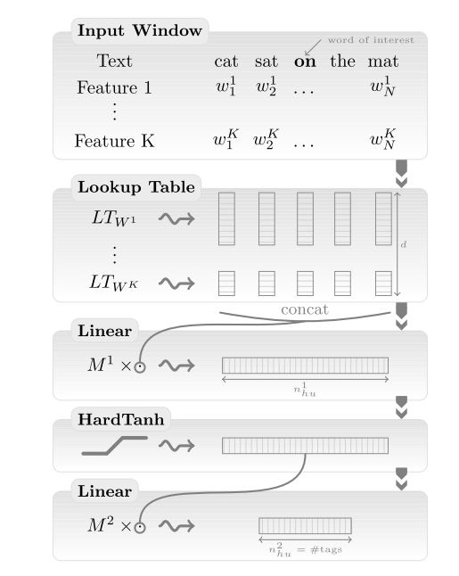
The resulting language model produces embeddings that already possess many of the relations word embeddings have become known for, e.g. countries are clustered close together and syntactically similar words occupy similar locations in the vector space. While their ranking objective eliminates the complexity of the softmax, they keep the intermediate fully-connected hidden layer (2.) of Bengio et al. around (the HardTanh layer in Figure 3), which constitutes another source of expensive computation. Partially due to this, their full model trains for seven weeks in total with \(|V| = 130000\).
Word2Vec
Let us now introduce arguably the most popular word embedding model, the model that launched a thousand word embedding papers: word2vec, the subject of two papers by Mikolov et al. in 2013. As word embeddings are a key building block of deep learning models for NLP, word2vec is often assumed to belong to the same group. Technically however, word2vec is not be considered to be part of deep learning, as its architecture is neither deep nor uses non-linearities (in contrast to Bengio's model and the C&W model).
In their first paper [7], Mikolov et al. propose two architectures for learning word embeddings that are computationally less expensive than previous models. In their second paper [8], they improve upon these models by employing additional strategies to enhance training speed and accuracy.
These architectures offer two main benefits over the C&W model and Bengio's language model:
- They do away with the expensive hidden layer.
- They enable the language model to take additional context into account.
As we will later show, the success of their model is not only due to these changes, but especially due to certain training strategies.
In the following, we will look at both of these architectures:
Continuous bag-of-words (CBOW)
While a language model is only able to look at the past words for its predictions, as it is evaluated on its ability to predict each next word in the corpus, a model that just aims to generate accurate word embeddings does not suffer from this restriction. Mikolov et al. thus use both the \(n\) words before and after the target word \( w_t \) to predict it as depicted in Figure 4. They call this continuous bag-of-words (CBOW), as it uses continuous representations whose order is of no importance.
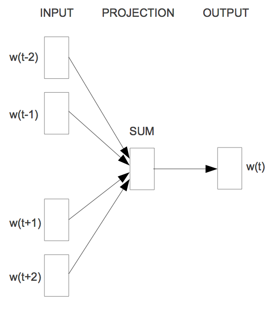
The objective function of CBOW in turn is only slightly different than the language model one:
\(J_\theta = \frac{1}{T}\sum\limits_{t=1}^T\ \text{log} \space p(w_t \: | \: w_{t-n} , \cdots , w_{t-1}, w_{t+1}, \cdots , w_{t+n})\).
Instead of feeding \( n \) previous words into the model, the model receives a window of \( n \) words around the target word \( w_t \) at each time step \( t \).
Skip-gram
While CBOW can be seen as a precognitive language model, skip-gram turns the language model objective on its head: Instead of using the surrounding words to predict the centre word as with CBOW, skip-gram uses the centre word to predict the surrounding words as can be seen in Figure 5.
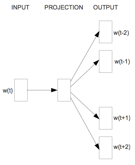
The skip-gram objective thus sums the log probabilities of the surrounding \( n \) words to the left and to the right of the target word \( w_t \) to produce the following objective:
\(J_\theta = \frac{1}{T}\sum\limits_{t=1}^T\ \sum\limits_{-n \leq j \leq n , \neq 0} \text{log} \space p(w_{t+j} \: | \: w_t)\).
To gain a better intuition of how the skip-gram model computes \( p(w_{t+j} \: | \: w_t) \), let's recall the definition of our softmax:
\(p(w_t \: | \: w_{t-1} , \cdots , w_{t-n+1}) = \dfrac{\text{exp}({h^\top v'_{w_t}})}{\sum_{w_i \in V} \text{exp}({h^\top v'_{w_i}})} \).
Instead of computing the probability of the target word \( w_t \) given its previous words, we calculate the probability of the surrounding word \( w_{t+j} \) given \( w_t \). We can thus simply replace these variables in the equation:
\(p(w_{t+j} \: | \: w_t ) = \dfrac{\text{exp}({h^\top v'_{w_{t+j}}})}{\sum_{w_i \in V} \text{exp}({h^\top v'_{w_i}})} \).
As the skip-gram architecture does not contain a hidden layer that produces an intermediate state vector \(h\), \(h\) is simply the word embedding \(v_{w_t}\) of the input word \(w_t\). This also makes it clearer why we want to have different representations for input embeddings \(v_w\) and output embeddings \(v'_w\), as we would otherwise multiply the word embedding by itself. Replacing \(h \) with \(v_{w_t}\) yields:
\(p(w_{t+j} \: | \: w_t ) = \dfrac{\text{exp}({v^\top_{w_t} v'_{w_{t+j}}})}{\sum_{w_i \in V} \text{exp}({v^\top_{w_t} v'_{w_i}})} \).
Note that the notation in Mikolov's paper differs slightly from ours, as they denote the centre word with \( w_I \) and the surrounding words with \( w_O \). If we replace \( w_t \) with \( w_I \), \( w_{t+j} \) with \( w_O \), and swap the vectors in the inner product due to its commutativity, we arrive at the softmax notation in their paper:
\(p(w_O|w_I) = \dfrac{\text{exp}(v'^\top_{w_O} v_{w_I})}{\sumV_{w=1}\text{exp}(v'\top_{w} v_{w_I})}\).
In the next post, we will discuss different ways to approximate the expensive softmax as well as key training decisions that account for much of skip-gram's success. We will also introduce GloVe [9], a word embedding model based on matrix factorisation and discuss the link between word embeddings and methods from distributional semantics.
Did I miss anything? Let me know in the comments below.
Citation
For attribution in academic contexts or books, please cite this work as:
Sebastian Ruder, "On word embeddings - Part 1". http://ruder.io/word-embeddings-1/, 2016.
BibTeX citation:
@misc{ruder2016wordembeddingspart1,
author = {Ruder, Sebastian},
title = {{On word embeddings - Part 1}},
year = {2016},
howpublished = {\url{http://ruder.io/word-embeddings-1/}},
}
Other blog posts on word embeddings
If you want to learn more about word embeddings, these other blog posts on word embeddings are also available:
- On word embeddings - Part 2: Approximating the softmax
- On word embeddings - Part 3: The secret ingredients of word2vec
- Unofficial Part 4: A survey of cross-lingual embedding models
- Unofficial Part 5: Word embeddings in 2017 - Trends and future directions
Translations
This blog post has been translated into the following languages:
Credit for the post image goes to Christopher Olah.
Bengio, Y., Ducharme, R., Vincent, P., & Janvin, C. (2003). A Neural Probabilistic Language Model. The Journal of Machine Learning Research, 3, 1137–1155. Retrieved from http://www.jmlr.org/papers/volume3/bengio03a/bengio03a.pdf ↩︎
Kim, Y., Jernite, Y., Sontag, D., & Rush, A. M. (2016). Character-Aware Neural Language Models. AAAI. Retrieved from http://arxiv.org/abs/1508.06615 ↩︎
Jozefowicz, R., Vinyals, O., Schuster, M., Shazeer, N., & Wu, Y. (2016). Exploring the Limits of Language Modeling. Retrieved from http://arxiv.org/abs/1602.02410 ↩︎
Chen, W., Grangier, D., & Auli, M. (2015). Strategies for Training Large Vocabulary Neural Language Models, 12. Retrieved from http://arxiv.org/abs/1512.04906 ↩︎
Collobert, R., & Weston, J. (2008). A unified architecture for natural language processing. Proceedings of the 25th International Conference on Machine Learning - ICML ’08, 20(1), 160–167. http://doi.org/10.1145/1390156.1390177 ↩︎
Collobert, R., Weston, J., Bottou, L., Karlen, M., Kavukcuoglu, K., & Kuksa, P. (2011). Natural Language Processing (almost) from Scratch. Journal of Machine Learning Research, 12 (Aug), 2493–2537. Retrieved from http://arxiv.org/abs/1103.0398 ↩︎
Mikolov, T., Corrado, G., Chen, K., & Dean, J. (2013). Efficient Estimation of Word Representations in Vector Space. Proceedings of the International Conference on Learning Representations (ICLR 2013), 1–12. ↩︎
Mikolov, T., Chen, K., Corrado, G., & Dean, J. (2013). Distributed Representations of Words and Phrases and their Compositionality. NIPS, 1–9. ↩︎
Pennington, J., Socher, R., & Manning, C. D. (2014). Glove: Global Vectors for Word Representation. Proceedings of the 2014 Conference on Empirical Methods in Natural Language Processing, 1532–1543. http://doi.org/10.3115/v1/D14-1162 ↩︎
