A survey of cross-lingual word embedding models
Monolingual word embeddings are pervasive in NLP. To represent meaning and transfer knowledge across different languages, cross-lingual word embeddings can be used. Such methods learn representations of words in a joint embedding space.

This post gives an overview of methods that learn a joint cross-lingual word embedding space between different languages.
Note: An updated version of this blog post is publicly available in the Journal of Artificial Intelligence Research.
In past blog posts, we discussed different models, objective functions, and hyperparameter choices that allow us to learn accurate word embeddings. However, these models are generally restricted to capture representations of words in the language they were trained on. The availability of resources, training data, and benchmarks in English leads to a disproportionate focus on the English language and a negligence of the plethora of other languages that are spoken around the world.
In our globalised society, where national borders increasingly blur, where the Internet gives everyone equal access to information, it is thus imperative that we do not only seek to eliminate bias pertaining to gender or race inherent in our representations, but also aim to address our bias towards language.
To remedy this and level the linguistic playing field, we would like to leverage our existing knowledge in English to equip our models with the capability to process other languages.
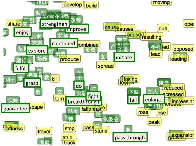
Perfect machine translation (MT) would allow this. However, we do not need to actually translate examples, as long as we are able to project examples into a common subspace such as the one in Figure 1.

Ultimately, our goal is to learn a shared embedding space between words in all languages. Equipped with such a vector space, we are able to train our models on data in any language. By projecting examples available in one language into this space, our model simultaneously obtains the capability to perform predictions in all other languages (we are glossing over some considerations here; for these, refer to this section). This is the promise of cross-lingual embeddings.
Over the course of this blog post, I will give an overview of models and algorithms that have been used to come closer to this elusive goal of capturing the relations between words in multiple languages in a common embedding space.
Note: While neural MT approaches implicitly learn a shared cross-lingual embedding space by optimizing for the MT objective, we will focus on models that explicitly learn cross-lingual word representations throughout this blog post. These methods generally do so at a much lower cost than MT and can be considered to be to MT what word embedding models (word2vec, GloVe, etc.) are to language modelling.
Types of cross-lingual embedding models
In recent years, various models for learning cross-lingual representations have been proposed. In the following, we will order them by the type of approach that they employ.
Note that while the nature of the parallel data used is equally discriminatory and has been shown to account for inter-model performance differences [1], we consider the type of approach more conducive to understanding the assumptions a model makes and -- consequently -- its advantages and deficiencies.
Cross-lingual embedding models generally use four different approaches:
- Monolingual mapping: These models initially train monolingual word embeddings on large monolingual corpora. They then learn a linear mapping between monolingual representations in different languages to enable them to map unknown words from the source language to the target language.
- Pseudo-cross-lingual: These approaches create a pseudo-cross-lingual corpus by mixing contexts of different languages. They then train an off-the-shelf word embedding model on the created corpus. The intuition is that the cross-lingual contexts allow the learned representations to capture cross-lingual relations.
- Cross-lingual training: These models train their embeddings on a parallel corpus and optimize a cross-lingual constraint between embeddings of different languages that encourages embeddings of similar words to be close to each other in a shared vector space.
- Joint optimization: These approaches train their models on parallel (and optionally monolingual data). They jointly optimise a combination of monolingual and cross-lingual losses.
In terms of parallel data, methods may use different supervision signals that depend on the type of data used. These are, from most to least expensive:
- Word-aligned data: A parallel corpus with word alignments that is commonly used for machine translation; this is the most expensive type of parallel data to use.
- Sentence-aligned data: A parallel corpus without word alignments. If not otherwise specified, the model uses the Europarl corpus consisting of sentence-aligned text from the proceedings of the European parliament that is generally used for training Statistical Machine Translation models.
- Document-aligned data: A corpus containing documents in different languages. The documents can be topic-aligned (e.g. Wikipedia) or label/class-aligned (e.g. sentiment analysis and multi-class classification datasets).
- Lexicon: A bilingual or cross-lingual dictionary with pairs of translations between words in different languages.
- No parallel data: No parallel data whatsoever. Learning cross-lingual representations from only monolingual resources would enable zero-shot learning across languages.
To make the distinctions clearer, we provide the following table, which serves equally as the table of contents and a springboard to delve deeper into the different cross-lingual models:
After the discussion of cross-lingual embedding models, we will additionally look into how to incorporate visual information into word representations, discuss the challenges that still remain in learning cross-lingual representations, and finally summarize which models perform best and how to evaluate them.
Monolingual mapping
Methods that employ monolingual mapping train monolingual word representations independently on large monolingual corpora. They then seek to learn a transformation matrix that maps representations in one language to the representations of the other language. They usually employ a set of source word-target word pairs that are translations of each other, which are used as anchor words for learning the mapping.
Note that all of the following methods presuppose that monolingual embedding spaces have already been trained. If not stated otherwise, these embedding spaces have been learned using the word2vec variants, skip-gram with negative sampling (SGNS) or continuous bag-of-words (CBOW) on large monolingual corpora.
Linear projection
Mikolov et al. have popularised the notion that vector spaces can encode meaningful relations between words. In addition, they notice that the geometric relations that hold between words are similar across languages [2], e.g. numbers and animals in English show a similar geometric constellation as their Spanish counterparts in Figure 2.

This suggests that it might be possible to transform one language's vector space into the space of another simply by utilising a linear projection with a transformation matrix \(W\).
In order to achieve this, they translate the 5,000 most frequent words from the source language and use these 5,000 translations pairs as bilingual dictionary. They then learn \(W\) using stochastic gradient descent by minimising the distance between the previously learned monolingual representations \(x_i\) of the source word \(w_i\) that is transformed using \(W\) and its translation \(z_i\) in the bilingual dictionary:
\(\min\limits_W \sum\limits^n_{i=1} |Wx_i - z_i|^2 \).
Projection via CCA
Faruqui and Dyer [3] propose to use another technique to learn the linear mapping. They use canonical correlation analysis (CCA) to project words from two languages into a shared embedding space. Different to linear projection, CCA learns a transformation matrix for every language, as can be seen in Figure 3, where the transformation matrix \(V\) is used to project word representations from the embedding space \(\Sigma\) to a new space \(\Sigma^\ast\), while \(W\) transforms words from \(\Omega\) to \(\Omega^\ast\). Note that \(\Sigma^\ast\) and \(\Omega^\ast\) can be seen as the same shared embedding space.

Similar to linear projection, CCA also requires a number of translation pairs in \(\Sigma'\) and \(\Omega'\) whose correlation can be maximised. Faruqui and Dyer obtain these pairs by selecting for each source word the target word to which it has been aligned most often in a parallel corpus. Alternatively, they could have also used a bilingual dictionary.
As CCA sorts the correlation vectors in \(V\) and \(W\) in descending order, Faruqui and Dyer perform experiments using only the top \(k\) correlated projection vectors and find that using the \(80\) % projection vectors with the highest correlation generally yields the highest performance.

Interestingly, they find that using multilingual projection helps to separate synonyms and antonyms in the source language, as can be seen in Figure 4, where the unprotected antonyms of "beautiful" are in two clusters in the top, whereas the CCA-projected vectors of the synonyms and antonyms form two distinct clusters in the bottom.
Normalisation and orthogonal transformation
Xing et al. [4] notice inconsistencies in the linear projection method by Mikolov et al. (2013), which they set out to resolve. Recall that Mikolov et al. initially learn monolingual word embeddings. For this, they use the skip-gram objective, which is the following:
\(\dfrac{1}{N} \sum\limits_{i=1}^N \sum\limits_{-C \leq j \leq C, j \neq 0} \text{log} P(w_{i+j} | w_i) \)
where \(C\) is the context length and \(P(w_{i+j} | w_i)\) is computed using the softmax:
\(P(w_{i+j} | w_i) = \dfrac{\text{exp}(c_{w_{i+j}}^T c_{w_i})}{\sum_w \text{exp}(c_w^T c_{w_i})}\).
They then learn a linear transformation between the two monolingual vector spaces with:
\(\text{min} \sum\limits_i |Wx_i - z_i|^2 \)
where \(W\) is the projection matrix that should be learned and \(x_i\) and \(z_i\) are word vectors in the source and target language respectively that are similar in meaning.
Xing et al. argue that there is a mismatch between the objective function used to learn word representations (maximum likelihood based on inner product), the distance measure for word vectors (cosine similarity), and the objective function used to learn the linear transformation (mean squared error), which may lead to degradation in performance.
They subsequently propose a method to resolve each of these inconsistencies: In order to fix the mismatch between the inner product similarity measure \(c_w^T c_{w'}\) during training and the cosine similarity measure \(\dfrac{c_w^T c_w'}{|c_w| |c_{w'}|}\) for testing, the inner product could also be used for testing. Cosine similarity, however, is used conventionally as an evaluation measure in NLP and generally performs better than the inner product. For this reason, they propose to normalise the word vectors to be unit length during training, which makes the inner product the same as cosine similarity and places all word vectors on a hypersphere as a side-effect, as can be seen in Figure 5.

They resolve the inconsistency between the cosine similarity measure now used in training and the mean squared error employed for learning the transformation by replacing the mean squared error with cosine similarity for learning the mapping, which yields:
\(\max\limits_W \sum\limits_i (Wx_i)^T z_i \).
Finally, in order to also normalise the projected vector \(Wx_i\) to be unit length, they constrain \(W\) to be an orthogonal matrix by solving a separate optimisation problem.
Max-margin and intruders
Lazaridou et al. [5] identify another issue with the linear transformation objective of Mikolov et al. (2013): They discover that using least-squares as objective for learning a projection matrix leads to hubness, i.e. some words tend to appear as nearest neighbours of many other words. To resolve this, they use a margin-based (max-margin) ranking loss (Collobert et al. [6]) to train the model to rank the correct translation vector \(y_i\) of a source word \(x_i\) that is projected to \(\hat{y_i}\) higher than any other target words \(y_j\):
\(\sum\limits^k_{j\neq i} \max \{ 0, \gamma + cos(\hat{y_i}, y_i) - cos(\hat{y_i}, y_j) \} \)
where \(k\) is the number of negative examples and \(\gamma\) is the margin.
They show that selecting max-margin over the least-squares loss consistently improves performance and reduces hubness. In addition, the choice of the negative examples, i.e. the target words compared to which the model should rank the correct translation higher, is important. They hypothesise that an informative negative example is an intruder ("truck" in the example), i.e. it is near the current projected vector \(\hat{y_i}\) but far from the actual translation vector \(y_i\) ("cat") as depicted in Figure 6.

These intruders should help the model identify cases where it is failing considerably to approximate the target function and should thus allow it to correct its behaviour. At every step of gradient descent, they compute \(s_j = cos(\hat{y_i}, y_j) - cos(y_i, y_j) \) for all vectors \(y_t\) in the target embedding space with \(j \neq i\) and choose the vector with the largest \(s_j\) as negative example for \(x_i\). Using intruders instead of random negative examples yields a small improvement of 2 percentage points on their comparison task.
Alignment-based projection
Guo et al. [7] propose another projection method that solely relies on word alignments. They count the number of times each word in the source language is aligned with each word in the target language in a parallel corpus and store these counts in an alignment matrix \(\mathcal{A}\).
In order to project a word \(w_i\) from its source representation \(v(w_i^S)\) to its representation in the target embedding space \(v(w_i)^T\) in the target embedding space, they simply take the average of the embeddings of its translations \(v(w_j)^T\) weighted by their alignment probability with the source word:
\(v(w_i)^T = \sum\limits_{i, j \in \mathcal{A}} \dfrac{c_{i, j}}{\sum_j c_{i,j}} \cdot v(w_j)^T\)
where \(c_{i,j}\) is the number of times the \(i^{th}\) source word has been aligned to the \(j^{th}\) target word.
The problem with this method is that it only assigns embeddings for words that are aligned in the reference parallel corpus. Gou et al. thus propagate alignments from in-vocabulary to OOV words by using edit distance as a metric for morphological similarity. They set the projected vector of an OOV source word \(v(w_{OOV}^T)\) as the average of the projected vectors of source words that are similar to it in edit distance:
\(v(w_{OOV}^T) = Avg(v(w_T))\)
where \(C = \{ w | EditDist(w_{OOV}^T, w) \leq \tau \} \). They set the threshold \(\tau\) empirically to \(1\).
Even though this approach seems simplistic, they actually observe significant improvements over projection via CCA in their experiments.
Multilingual CCA
Ammar et al. [8] extend the bilingual CCA projection method of Faruqui and Dyer (2014) to the multi-lingual setting using the English embedding space as the foundation for their multilingual embedding space.
They learn the two projection matrices for every other language with English. The transformation from each target language space \(\Omega\) to the English embedding space \(\Sigma\) can then be obtained by projecting the vectors in \(\Omega\) into the CCA space \(\Omega^\ast\) using the transformation matrix \(W\) as in Figure 3. As \(\Omega^\ast\) and \(\Sigma^\ast\) lie in the same space, vectors in \(\Sigma^\ast\) can be projected into the English embedding space \(\Sigma\) using the inverse of \(V\).
Hybrid mapping with symmetric seed lexicon
The previous mapping approaches used a bilingual dictionary as inherent component of their model, but did not pay much attention to the quality of the dictionary entries, using either automatic translations of frequent words or word alignments of all words.
Vulić and Korhonen [9] in turn emphasise the role of the seed lexicon that is used for learning the projection matrix. They propose a hybrid model that initially learns a first shared bilingual embedding space based on an existing cross-lingual embedding model. They then use this initial vector space to obtain translations for a list of frequent source words by projecting them into the space and using the nearest neighbour in the target language as translation. With these translation pairs as seed words, they learn a projection matrix analogously to Mikolov et al. (2013).
In addition, they propose a symmetry constraint, which enforces that words are only included if their projections are neighbours of each other in the first embedding space. Additionally, one can retain pairs whose second nearest neighbours are less similar than the first nearest neighbours up to some threshold.
They run experiments showing that their model with the symmetry constraint outperforms comparison models and that a small threshold of \(0.01\) or \(0.025\) leads to slightly improved performance.
Orthogonal transformation, normalisation, and mean centering
The previous approaches have introduced models that imposed different constraints for mapping monolingual representations of different languages to each other. The relation between these methods and constraints, however, is not clear.
Artetxe et al. [10] thus propose to generalise previous work on learning a linear transformation between monolingual vector spaces: Starting with the basic optimisation objective, they propose several constraints that should intuitively help to improve the quality of the learned cross-lingual representations. Recall that the linear transformation learned by Mikolov et al. (2013) aims to find a parameter matrix \(W\) that satisfies:
\(\DeclareMathOperator*{\argmin}{argmin} \argmin\limits_W \sum\limits_i |Wx_i - z_i|^2 \)
where \(x_i\) and \(z_i\) are similar words in the source and target language respectively.
If the performance of the embeddings on a monolingual evaluation task should not be degraded, the dot products need to be preserved after the mapping. This can be guaranteed by requiring \(W\) to be an orthogonal matrix.
Secondly, in order to ensure that all embeddings contribute equally to the objective, embeddings in both languages can be normalised to be unit vectors:
\(\argmin\limits_W \sum\limits_i | W \dfrac{x_i}{|x_i|} - \dfrac{z_i}{|z_i|}|^2 \).
As the norm of an orthogonal matrix is \(1\), if \(W\) is orthogonal, we can add it to the denominator and move \(W\) to the numerator:
\(\argmin\limits_W \sum\limits_i | \dfrac{Wx_i}{|Wx_i|} - \dfrac{z_i}{|z_i|}|^2 \).
Through expansion of the above binomial, we obtain:
\(\argmin\limits_W \sum\limits_i |\dfrac{Wx_i}{|Wx_i|}|^2 + |\dfrac{z_i}{|z_i||}|^2 - 2 \dfrac{Wx_i}{|Wx_i|}^T \dfrac{z_i}{|z_i|} \).
As the norm of a unit vector is \(1\) the first two terms reduce to \(1\), which leaves us with the following:
\(\argmin\limits_W \sum\limits_i 2 - 2 \dfrac{Wx_i}{|Wx_i|}^T \dfrac{z_i}{|z_i|} ) \).
The latter term now is just the cosine similarity of \(Wx_i\) and \(z_i\):
\(\argmin\limits_W \sum\limits_i 2 - 2 \text{cos}(Wx_i, z_i) \).
As we are interested in finding parameters \(W\) that minimise our objective, we can remove the constants above:
\(\argmin\limits_W \sum\limits_i - \text{cos}(Wx_i, z_i) \).
Minimising the sum of negative cosine similarities is then equal to maximising the sum of cosine similarities, which gives us the following:
\(\DeclareMathOperator*{\argmax}{argmax} \argmax\limits_W \sum\limits_i \text{cos}(Wx_i, z_i) \).
This is equal to the objective by Xing et al. (2015), although they motivated it via an inconsistency of the objectives.
Finally, Artetxe et al. argue that two randomly selected words are generally expected not to be similar. For this reason, the cosine of their embeddings in any dimension -- as well as their cosine similarity -- should be zero. They capture this intuition by performing dimension-wise mean centering with a centering matrix \(C_m\):
\(\argmin\limits_W \sum\limits_i ||C_mWx_i - C_mz_i||^2 \).
This reduces to maximizing the sum of dimension-wise covariance as long as \(W\) is orthogonal similar as above:
\(\argmax\limits_W \sum\limits_i \text{cov}(Wx_i, z_i) \).
Interestingly, the method by Faruqui and Dyer (2014) is similar to this objective, as CCA maximizes the dimension-wise covariance of both projections. This is equivalent to the single projection here, as it is constrained to be orthogonal. The only difference is that, while CCA changes the monolingual embeddings so that different dimensions have the same variance and are uncorrelated -- which might degrade performance -- Artetxe et al. enforce monolingual invariance.
Adversarial auto-encoder
All previous approaches to learning a transformation matrix between monolingual representations in different languages require either a dictionary or word alignments as a source of parallel data.
Barone [11], in contrast, seeks to get closer to the elusive goal of creating cross-lingual representations without parallel data. He proposes to use an adversarial auto-encoder to transform source embeddings into the target embedding space. The auto-encoder is then trained to reconstruct the source embeddings, while the discriminator is trained to differentiate the projected source embeddings from the actual target embeddings as in Figure 7.

While intriguing, learning a transformation between languages without any parallel data at all seems unfeasible at this point. However, future approaches that aim to learn a mapping with fewer and fewer parallel data may bring us closer to this goal.
More generally, however, it remains unclear if a projection can reliably transform the embedding space of one language into the embedding space of another language. Additionally, the reliance on lexicon data or word alignment information is expensive.
Pseudo-cross-lingual
The second type of cross-lingual models seeks to construct a pseudo-cross-lingual corpus that captures interactions between the words in different languages. Most approaches aim to identify words that can be translated to each other in monolingual corpora of different languages and replace these with placeholders to ensure that translations of the same word have the same vector representation.
Mapping of translations to same representation
Xiao and Guo [12] propose the first pseudo-cross-lingual method that leverages translation pairs: They first translate all words that appear in the source language corpus into the target language using Wiktionary. As these translation pairs are still very noisy, they filter them by removing polysemous words in the source and target language and translations that do not appear in the target language corpus. From this bilingual dictionary, they now create a joint vocabulary, in which each translation pair has the same vector representation.
For training, they use the margin-based ranking loss of Collobert et al. (2008) to rank correct word windows higher than corrupted ones, where the middle word is replaced by an arbitrary word.
In contrast to the subsequent methods, they do not construct a pseudo-cross-lingual corpus explicitly. Instead, they feed windows of both the source and target corpus into the model during training, thereby essentially interpolating source and target language.
It is thus most likely that, for ease of training, the authors replace translation pairs in source and target corpus with a placeholder to ensure a common vector representation, similar to the procedure of subsequent models.
Random translation replacement
Gouws and Søgaard [13] in turn explicitly create a pseudo-cross-lingual corpus: They leverage translation pairs of words in the source and in the target language obtained via Google Translate. They concatenate the source and target corpus and replace each word that is part of a translation pair with its translation equivalent with a probability of 50%. They then train CBOW on this corpus.
It is interesting to note that they also experiment with replacing words not based on translation but part-of-speech equivalence, i.e. words with the same part-of-speech in different languages will be replaced with one another. While replacement based on part-of-speech leads to small improvements for cross-lingual part-of-speech tagging, replacement based on translation equivalences yields even better performance for the task.
On-the-fly replacement and polysemy handling
Duong et al. [14] propose a similar approach to Gouws and Søgaard (2015). They also use CBOW, which predicts the centre word in a window given the surrounding words. Instead of randomly replacing every word in the corpus with its translation during pre-processing, they replace each centre word with a translation on-the-fly during training.
In addition to past approaches, they also seek to handle polysemy explicitly by proposing an EM-inspired method that chooses as replacement the translation \(\bar{w_i}\) whose representation is most similar to the combination of the representations of the source word \(v_{w_i}\) and the context vector \(h_i\):
\(\bar{w_i} = \text{argmax}_{w \in \text{dict}(w_i)} \text{cos}(v_{w_i} + h_i, v_w) \)
where \(\text{dict}(w_i)\) contains the translations of \(w_i\).
They then jointly learn to predict both the words and their appropriate translations. They use PanLex as bilingual dictionary, which covers around 1,300 language with about 12 million expressions. Consequently, translations are high coverage but often noisy.
Multilingual cluster
Ammar et al. (2016) propose another approach that is similar to the previous method by Gouws and Søgaard (2015): They use bilingual dictionaries to find clusters of synonymous words in different languages. They then concatenate the monolingual corpora of different languages and replace tokens in the same cluster with the cluster ID. They then train SGNS on the concatenated corpus.
Document merge and shuffle
The previous methods all use a bilingual dictionary or a translation tool as a source of translation pairs that can be used for replacement.
Vulić and Moens [15] present a model that does without translation pairs and learns cross-lingual embeddings only from document-aligned data. In contrast to the previous methods, the authors propose not to merge two monolingual corpora but two aligned documents of different languages into a pseudo-bilingual document.
They concatenate the documents and then shuffle them by randomly permutating the words. The intuition is that as most methods rely on learning word embeddings based on their context, shuffling the documents would lead to bilingual contexts for each word that will enable the creation of a robust embedding space. As shuffling is necessarily random, however, it might lead to sub-optimal configurations.
For this reason, they propose another merging strategy that assumes that the structures of the document are similar: They then alternatingly insert words from each language into the pseudo-bilingual document in the order in which they appear in their monolingual document and based on the mono-lingual documents' length ratio.
While pseudo-cross-lingual approaches are attractive due to their simplicity and ease of implementation, relying on naive replacement and permutation does not allow them to capture more sophisticated facets of cross-lingual relations.
Cross-lingual training
Cross-lingual training approaches focus exclusively on optimising the cross-lingual objective. These approaches typically rely on sentence alignments rather than a bilingual lexicon and require a parallel corpus for training.
Bilingual compositional sentence model
The first approach that optimizes only a cross-lingual objective is the bilingual compositional sentence model by Hermann and Blunsom [16]. They train two models to produce sentence representations of aligned sentences in two languages and use the distance between the two sentence representations as objective. They minimise the following loss:
\(E_{dist}(a,b) = |a_{\text{root}} - b_{\text{root}} |^2 \)
where \(a_{\text{root}}\) and \(b_{\text{root}}\) are the representations of two aligned sentences from different languages. They compose \(a_{\text{root}}\) and \(b_{\text{root}}\) simply as the sum of the embeddings of the words in the corresponding sentence. The full model is depicted in Figure 8.

They train the model then to output a higher score for correct translations than for randomly sampled incorrect translations using the max-margin hinge loss of Collobert et al. (2008).
Bilingual bag-of-words autoencoder
Instead of minimising the distance between two sentence representations in different languages, Lauly et al. [17] aim to reconstruct the target sentence from the original source sentence. They start with a monolingual autoencoder that encodes an input sentence as a sum of its word embeddings and tries to reconstruct the original source sentence. For efficient reconstruction, they opt for a tree-based decoder that is similar to a hierarchical softmax. They then augment this autoencoder with a second decoder that reconstructs the aligned target sentence from the representation of the source sentence as in Figure 9.

Encoders and decoders have language-specific parameters. For an aligned sentence pair, they then train the model with four reconstruction losses: for each of the two sentences, they reconstruct from the sentence to itself and to its equivalent in the other language.
Distributed word alignment
While the previous approaches required word alignments as a prerequisite for learning cross-lingual embeddings, Kočiský et al. [18] simultaneously learn word embeddings and alignments. Their model, Distributed Word Alignment, combines a distributed version of FastAlign (Dyer et al. [19]) with a language model. Similar to other bilingual approaches, they use the word in the source language sentence of an aligned sentence pair to predict the word in the target language sentence.
They replace the standard multinomial translation probability of FastAlign with an energy function that tries to bring the representation of a target word \(f\) close to the sum of the context words around the word \(e_i\) in the source sentence:
\(E(f, e_i) = - ( \sum\limits_{s=-k}^k r^T_{e_{i+s}} T_s) r_f - b_r^T r_f - b_f \)
where \(r_{e_{i+s}}\) and \(r_f\) are vector representations for source and target words, \(T_s\) is a projection matrix, and \(b_r\) and \(b_f\) are representation and target biases respectively. For calculating the translation probability \(p(f|e_i)\), we then simply need to apply the softmax to the translation probabilities between the source word and all words in the target language.
In addition, the authors speed up training by using a class factorisation strategy similar to the hierarchical softmax and predict frequency-based class representations instead of word representations. For training, they also use EM but fix the alignment counts learned by FastAlign that was initially trained for 5 epochs during the E-step and optimise the translation probabilities in the M-step only.
Bilingual compositional document model
Hermann and Blunsom [20] extend their approach (Hermann and Blunsom, 2013) to documents, by applying their composition and objective function recursively to compose sentences into documents. First, sentence representations are computed as before. These sentence representations are then fed into a document-level compositional vector model, which integrates the sentence representations in the same way as can be seen in Figure 10.

The advantage of this method is that weaker supervision in the form of document-level alignment can be used instead of or in conjunction with sentence-level alignment. The authors run experiments both on Europarl as well as on a newly created corpus of multilingual aligned TED talk transcriptions and find that the document signal helps considerably.
In addition, they propose another composition function that -- instead of summing the representations -- applies a non-linearity to bigram pairs:
\(f(x) = \sum\limits_{i=1}^n \text{tanh}(x_{i-1} + x_i)\)
They find that this composition slightly outperforms addition, but underperforms it on smaller training datasets.
Bag-of-words autoencoder with correlation
Chandar et al. [21] extend the approach by Lauly et al. (2013) in two ways: Instead of using a tree-based decoder for calculating the reconstruction loss, they reconstruct a sparse binary vector of word occurrences as in Figure 11. Due to the high-dimensionality of the binary bag-of-words vector, reconstruction is slower. As they perform training using mini-batch gradient descent, where each mini-batch consists of adjacent sentences, they propose to merge the bags-of-words of the mini-batch into a single bag-of-words and to perform updates based on the merged bag-of-words. They find that this yields good performance and even outperforms the tree-based decoder.

Secondly, they propose to add a term \(cor(a(x), a(y))\) to the objective function that encourages correlation between the representations \(a(x)\) , \(a(y)\) of the source and target language respectively by summing the scalar correlations between all dimensions of the two vectors.
Bilingual paragraph vectors
Similar to the previous methods, Pham et al. [22] learn sentence representations as a means for learning cross-lingual word embeddings. They extend paragraph vectors (Mikolov et al. [23]) to the multilingual setting by forcing aligned sentences of different languages to share the same vector representation as in Figure 12 where \(sent\) is the shared sentence representation. The shared sentence representation is concatenated with the sum of the previous \(N\) words in the sentence and the model is trained to predict the next word in the sentence.

The authors use a hierarchical softmax to speed-up training. As the model only learns representations for the sentences it has seen during training, at test time for an unknown sentence, the sentence representation is randomly initialised and the model is trained to predict only the words in the sentence. Only the sentence vector is updated, while the other model parameters are frozen.
Translation-invariant LSA
Besides word embedding models such as skip-gram, matrix factorisation approaches have historically been used successfully to learn representations of words. One of the most popular methods is LSA, which Gardner et al. [24] extend as translation-invariant LSA to to learn cross-lingual word embeddings. They factorise a multilingual co-occurrence matrix with the restriction that it should be invariant to translation, i.e. it should stay the same if multiplied with the respective word or context dictionary.
Inverted indexing on Wikipedia
All previous approaches to learn cross-lingual representations have been based on some form of language model or matrix factorisation. In contrast, Søgaard et al. [25] propose an approach that does without any of these methods, but instead relies on the structure of the multilingual knowledge base Wikipedia, which they exploit by inverted indexing. Their method is based on the intuition that similar words will be used to describe the same concepts across different languages.
In Wikipedia, articles in multiple languages deal with the same concept. We would typically represent every concept with the terms that are used to describe it across different languages. To learn cross-lingual word representations, we can now simply invert the index and instead represent a word by the Wikipedia concepts it is used to describe. This way, we are directly provided with cross-lingual representations of words without performing any optimisation whatsoever. As a post-processing step, we can perform dimensionality reduction on the produced word representations.
While the previous methods are able to make effective use of parallel sentence and documents to learn cross-lingual word representations, they neglect the monolingual quality of the learned representations. Ultimately, we do not only want to embed languages into a shared embedding space, but also want the monolingual representations do well on the task at hand.
Joint optimisation
Models that use joint optimisation aim to do exactly this: They not only consider a cross-lingual constraint, but jointly optimize mono-lingual and cross-lingual objectives.
In practice, for two languages \(l_1\) and \(l_2\), these models optimize a monolingual loss \(\mathcal{M}\) for each language and one or multiple terms \(\Omega\) that regularize the transfer from language \(l_1\) to \(l_2\) (and vice versa):
\(\mathcal{M}_{l_1} + \mathcal{M}_{l_2} + \lambda (\Omega_{l_1 \rightarrow l_2} + \Omega_{l_2 \rightarrow l_1}) \)
where \(\lambda\) is an interpolation parameter that adjusts the impact of the cross-lingual regularization.
Multi-task language model
The first jointly optimised model for learning cross-lingual representations was created by Klementiev et al. [26]. They train a neural language model for each language and jointly optimise the monolingual maximum likelihood objective of each language model with a word-alignment based MT regularization term as the cross-lingual objective. The monolingual objective is thus to maximise the probability of the current word \(w_t\) given its \(n\) surrounding words:
\(\mathcal{M} = \text{log} P(w_t^ | w_{t-n+1:t-1}) \).
This is optimised using the classic language model of Bengio et al. [27]. The cross-lingual regularisation term in turn encourages the representations of words that are often aligned to each other to be similar:
\(\Omega = \dfrac{1}{2} c^T (A \otimes I) c\)
where \(A\) is the matrix capturing alignment scores, \(I\) is the identity matrix, \(\otimes\) is the Kronecker product, and \(c\) is the representation of word \(w_t\).
Bilingual matrix factorisation
Zou et al. [28] use a matrix factorisation approach in the spirit of GloVe (Pennington et al. [29]) to learn cross-lingual word representations for English and Chinese. They create two alignment matrices \(A_{en \rightarrow zh}\) and \(A_{zh \rightarrow en}\) using alignment counts automatically learned from the Chinese Gigaword corpus. In \(A_{en \rightarrow zh}\), each element \(a_{ij}\) contains the number of times the \(i\)-th Chinese word was aligned with the \(j\)-th English word, with each row normalised to sum to \(1\).
Intuitively, if a word in the source language is only aligned with one word in the target language, then those words should have the same representation. If the target word is aligned with more than one source word, then its representation should be a combination of the representations of its aligned words. Consequently, the authors represent the embeddings in the target language as the product of the source embeddings \(V_{en}\) and their corresponding alignment counts \(A_{en \rightarrow zh}\). They then minimise the squared difference between these two terms:
\(\Omega_{en\rightarrow zh} = || V_{zh} - A_{en \rightarrow zh} V_{en}||^2 \)
\(\Omega_{zh\rightarrow en} = || V_{en} - A_{zh \rightarrow en} V_{zh}||^2 \)
where \(V_{en}\) and \(V_{zh}\) are the embedding matrices of the English and Chinese word embeddings respectively.
They employ the max-margin hinge loss objective by Collobert et al. (2008) as monolingual objective \(\mathcal{M}\) and train the English and Chinese word embeddings to minimise the corresponding objective above together with a monolingual objective. For instance, for English, the training objective is:
\(\mathcal{M}_{en} + \lambda \Omega_{zh\rightarrow en} \).
It is interesting to observe that the authors learn embeddings using a curriculum, training different frequency bands of the vocabulary at a time. The entire training process takes 19 days.
Bilingual skip-gram
Luong et al. [30] in turn extend skip-gram to the cross-lingual setting and use the skip-gram objectives as monolingual and cross-lingual objectives. Rather than just predicting the surrounding words in the source language, they use the words in the source language to additionally predict their aligned words in the target language as in Figure 13.

For this, they require word alignment information. They propose two ways to predict aligned words: For their first method, they automatically learn alignment information; if a word is unaligned, the alignments of its neighbours are used for prediction. In their second method, they assume that words in the source and target sentence are monotonically aligned, with each source word at position \(i\) being aligned to the target word at position \(i \cdot T/S\) where \(S\) and \(T\) are the source and target sentence lengths. They find that a simple monotonic alignment is comparable to the unsupervisedly learned alignment in performance.
Bilingual bag-of-words without word alignments
Gouws et al. [31] propose a Bilingual Bag-of-Words without Word Alignments (BilBOWA) that leverages additional monolingual data. They use the skip-gram objective as a monolingual objective and a novel sampled \(l_2\) loss as cross-lingual regularizer as in Figure 14.

More precisely, instead of relying on expensive word alignments, they simply assume that each word in a source sentence is aligned with every word in the target sentence under a uniform alignment model. Thus, instead of minimising the distance between words that were aligned to each other, they minimise the distance between the means of the word representations in the aligned sentences, which is shown in Figure 15, where \(s^e\) and \(s^f\) are the sentences in source and target language respectively.

The cross-lingual objective in the BilBOWA model is thus:
\(\Omega = |\dfrac{1}{m} \sum\limits_{w_i \in s{l_1}}m r_i^{l_1} - \dfrac{1}{n} \sum\limits_{w_j \in s{l_2}}n r_j^{l_2}
|^2 \)
where \(r_i\) and \(r_j\) are the word embeddings of word \(w_i\) and \(w_j\) in each sentence \(s^{l_1}\) and \(s^{l_2}\) of length \(m\) and \(n\) in languages \(l_1\) and \(l_2\) respectively.
Bilingual skip-gram without word alignments
Another extension of skip-gram to learning cross-lingual representations is proposed by Coulmance et al. [32]. They also use the regular skip-gram objective as monolingual objective. For the cross-lingual objective, they make a similar assumption as Gouws et al. (2015) by supposing that every word in the source sentence is uniformly aligned to every word in the target sentence.
Under the skip-gram formulation, they treat every word in the target sentence as context of every word in the source sentence and thus train their model to predict all words in the target sentence with the following skip-gram objective:
\(\Omega_{e,f} = \sum\limits_{(s_{l_1}, s_{l_2}) \in C_{l_1, l_2}} \sum\limits_{w_{l_1} \in s_{l_1}} \sum\limits_{c_{l_2} \in s_{l_2}} - \text{log} \sigma(w_{l_1}, c_{l_2}) \)
where \(s\) is the sentence in the respective language, \(C\) is the sentence-aligned corpus, \(w\) are word and \(c\) are context representations respectively, and \( - \text{log} \sigma(\centerdot)\) is the standard skip-gram loss function.
As the cross-lingual objective is asymmetric, they use one cross-lingual objective for the source-to-target and another one for the target-to-source direction. The complete Trans-gram objective including two monolingual and two cross-lingual skip-gram objectives is displayed in Figure 16.
Joint matrix factorisation
Shi et al. [33] use a joint matrix factorisation model to learn cross-lingual representations. In contrast to Zou et al. (2013), they also take into account additional monolingual data. Similar to the former, they also use the GloVe objective (Pennington et al., 2014) as monolingual objective:
\(\mathcal{M}_{l_i} = \sum\limits_{j,k} f(X_{jk}{l_i})(w_j{l_i} \cdot c_k^{l_i} + b_{w_j}^{l_i} + b_{c_k}^{l_i} + b^{l_i} - M_{jk}^{l_{i}}) \)
where \(w_j^{l_i}\) and \(c_k^{l_i}\) are the embeddings and \(M_{jk}^{l_{i}}\) the PMI value of a word-context pair \((j,k) \) in language \(l_{i}\), while \( b_{w_j}^{l_i}\) and \(b_{c_k}^{l_i}\) and \(b^{l_i}\) are the word-specific and language-specific bias terms respectively.

They then place cross-lingual constraints on the monolingual representations as can be seen in Figure 17. The authors propose two cross-lingual regularisation objectives: The first one is based on calculating cross-lingual co-occurrence counts. These co-occurrences can be calculated without alignment information using a uniform alignment model as in Gouws et al. (2015). Alternatively, co-occurrence counts can also be calculated by leveraging automatically learned word alignments. The co-occurrence counts are then stored in a matrix \(X^{\text{bi}}\) where every entry \(X_{jk}^{\text{bi}}\) contains the number of times the source word \(j\) occurred with the target word \(k\) in an aligned sentence pair in the parallel corpus.
For optimisation, a PMI matrix \(M^{\text{bi}}_{jk}\) can be calculated based on the co-occurrence counts in \(X^{\text{bi}}\). This matrix can again be factorised as in the GloVe objective, where now the context word representation \(c_k^{l_i}\) is replaced with the representation of the word in the target language \(w_k^{l_2}\):
\(\Omega = \sum\limits_{j \in V^{l_1}, k \in V^{l_2}} f(X_{jk}{l_1})(w_j{l_1} \cdot w_k^{l_2} + b_{w_j}^{l_1} + b_{w_k}^{l_2} + b^{\text{bi}} - M_{jk}^{\text{bi}}) \).
The second cross-lingual regularisation term they propose leverages the translation probabilities produced by a machine translation system and involves minimising the distances of the representations of related words in the two languages weighted by their similarities:
\(\Omega = \sum\limits_{j \in V^{l_1}, k \in V^{l_2}} sim(j,k) \cdot ||w_j^{l_1} - w_k{l_2}||2\)
where \(j\) and \(k\) are words in the source and target language respectively and \(sim(j,k)\) is their translation probability.
Bilingual sparse representations
Vyas and Carpuat [34] propose another method based on matrix factorisation that -- in contrast to previous approaches -- allows learning sparse cross-lingual representations. They first independently train two monolingual word representations \(X_e\) and \(X_f\) in two different languages using GloVe (Pennington et al., 2014) on two large monolingual corpora.
They then learn monolingual sparse representations from these dense representations by decomposing \(X\) into two matrices \(A\) and \(D\) such that the \(l_2\) reconstruction error is minimised, with an additional constraint on \(A\) for sparsity:
\(\mathcal{M}_{l_i} = \sum\limits_{i=1}^{v_{l_i}} |A_{l_ii}D_{l_i}^T - X_{l_ii}| + \lambda_{l_i} |A_{l_ii}|_1 \)
where \(v_{l_i}\) is the number of dense word representations in language \(l_i\).
The above equation, however, only creates sparse monolingual embeddings. To learn bilingual embeddings, they add another constraint based on automatically learned word alignment that minimises the \(l_2\) reconstruction error between words that were strongly aligned to each other:
\(\Omega = \sum\limits_{i=1}^{v_{l_1}} \sum\limits_{j=1}^{v_{l_2}} \dfrac{1}{2} \lambda_x S_{ij} |A_{l_1i} - A_{l_2j}|_2^2 \)
where \(S\) is the alignment matrix where each entry \(S_{ij}\) contains the alignment score of source word \(X_{l_1i}\) with target word \(X_{l_2j}\).
The complete objective function is thus the following:
\(\mathcal{M}_{l_1} + \mathcal{M}_{l_2} + \Omega\).
Bilingual paragraph vectors (without parallel data)
Mogadala and Rettinger [35] use an approach similar to Pham et al. (2015), but extend it to also work without parallel data. They use the paragraph vectors objective as monolingual objective \(\mathcal{M}\). They jointly optimise this objective together with a cross-lingual regularization function \(\Omega\) that encourages the representations of words in languages \(l_1\) and \(l_2\) to be close to each other.
Their main innovation is that the cross-lingual regularizer \(\Omega\) is adjusted based on the nature of the training corpus. In addition to regularising the mean of word vectors in a sentence to be close to the mean of word vectors in the aligned sentence similar to Gouws et al. (2015) (the second term in the below equation), they also regularise the paragraph vectors \(SP^{l_1}\) and \(SP^{l_2}\) of aligned sentences in languages \(l_1\) and \(l_2\) to be close to each other. The complete cross-lingual objective then uses elastic net regularization to combine both terms:
\(\Omega = \alpha ||SP^{l_1}_j - SP{l_2}_j||2 + (1-\alpha) \dfrac{1}{m} \sum\limits_{w_i \in s_j{l_1}}m W_i^{l_1} - \dfrac{1}{n} \sum\limits_{w_k \in s_j{l_2}}n W_k^{l_2} \)
where \(W_i^{l_1}\) and \(W_k^{l_2}\) are the word embeddings of word \(w_i\) and \(w_k\) in each sentence \(s_j\) of length \(m\) and \(n\) in languages \(l_1\) and \(l_2\) respectively.
To leverage data that is not sentence-aligned, but where an alignment is still present on the document level, they propose a two-step approach: They use Procrustes analysis, a method for statistical shape analysis, to find for each document in language \(l_1\) the most similar document in language \(l_2\). This is done by first learning monolingual representations of the documents in each language using paragraph vectors on each corpus. Subsequently, Procrustes analysis aims to learn a transformation between the two vector spaces by translating, rotating, and scaling the embeddings in the first space until they most closely align to the document representations in the second space.
In the second step, they then simply use the previously described method to learn cross-lingual word representations from the alignment documents, this time treating the entire documents as paragraphs.
Incorporating visual information
A recent branch of research proposes to incorporate visual information to improve the performance of monolingual [36] or cross-lingual [37] representations. These methods show good performance on comparison tasks. They additionally demonstrate application for zero-shot learning and might thus ultimately be helpful in learning cross-lingual representations without (linguistic) parallel data.
Challenges
Functional modeling
Models for learning cross-linguistic representations share weaknesses with other vector space models of language: While they are very good at modelling the conceptual aspect of meaning evaluated in word similarity tasks, they fail to properly model the functional aspect of meaning, e.g. to distinguish whether one remarks "Give me a pencil" or "Give me that pencil".
Word order
Secondly, due to the reliance on bag-of-words representations, current models for learning cross-lingual word embeddings completely ignore word order. Models that are oblivious to word order, for instance, assign to the following sentence pair (Landauer & Dumais [38]) the exact same representation as they contain the same set of words, even though they are completely different in meaning:
- "That day the office manager, who was drinking, hit the problem sales worker with a bottle, but it was not serious."
- "It was not the sales manager, who hit the bottle that day, but the office worker with a serious drinking problem".
Compositionality
Most approaches for learning cross-lingual representations focus on word representations. These approaches are not able to easily compose word representations to form representations of sentences and documents. Even approaches that learn jointly learn word and sentence representations do so by via simple summation of words in the sentence. In the future, it will be interesting to see if LSTMs or CNNs that can form more composable sentence representations can be applied efficiently to learn cross-lingual representations.
Polysemy
While conflating multiple senses of a word is already problematic for learning mono-lingual word representations, this issue is amplified in a cross-lingual embedding space: Monosemous words in one language might align with polysemous words in another language and thus fail to capture the entirety of the cross-lingual relations. There has already been promising work on learning monolingual multi-sense embeddings. We hypothesize that learning cross-lingual multi-sense embeddings will become increasingly relevant, as it enables us to capture more fine-grained cross-lingual meaning.
Feasibility
The final challenge pertains to the feasibility of the venture of learning cross-lingual embeddings itself: Languages are incredibly complex, human artefacts. Learning a monolingual embedding space is already difficult; sharing such a vector space between two languages and expecting that inter-language and intra-language relations are reliably reflected then seems utopian.
Additionally, some languages show linguistic features, which other languages lack. The ease of constructing a shared embedding space between languages and consequently the success of cross-lingual transfer is intuitively proportional to the similarity of the languages: An embedding space shared between Spanish and Portuguese tends to capture more linguistic nuances of meaning than an embedding space populated with English and Chinese representations. Furthermore, if two languages are too dissimilar, cross-linguistic transfer might not be possible at all -- similar to the negative transfer that occurs in domain adaptation between very dissimilar domains.
Evaluation
Having surveyed models to learn cross-lingual word representations, we would now like to know which is the best method to use for the task we care about. Cross-lingual representation models have been evaluated on a wide range of tasks such as cross-lingual document classification (CLDC), Machine Translation (MT), word similarity, as well as cross-lingual variations of the following tasks: named entity recognition, part-of-speech tagging, super sense tagging, dependency parsing, and dictionary induction.
In the context of the CLDC evaluation setup by Klementiev et al. (2012) \(40\)-dimensional cross-lingual word embeddings are learned to classify documents in one language and evaluated on the documents of another language. As CLDC is among the most widely used, we show below exemplarily the evaluation table of Mogadala and Rettinger (2016) for this task:
| Method | en -> de | de -> en | en -> fr | fr -> en | en -> es | es -> en |
|---|---|---|---|---|---|---|
| Majority class | 46.8 | 46.8 | 22.5 | 25.0 | 15.3 | 22.2 |
| MT | 68.1 | 67.4 | 76.3 | 71.1 | 52.0 | 58.4 |
| Multi-task language model (Klementiev et al., 2012) | 77.6 | 71.1 | 74.5 | 61.9 | 31.3 | 63.0 |
| Bag-of-words autoencoder with correlation (Chandar et al., 2014) | 91.8 | 74.2 | 84.6 | 74.2 | 49.0 | 64.4 |
| Bilingual compositional document model (Hermann and Blunsom, 2014) | 86.4 | 74.7 | - | - | - | - |
| Distributed word alignment (Kočiský et al., 2014) | 83.1 | 75.4 | - | - | - | - |
| Bilingual bag-of-words without word alignments (Gouws et al., 2015) | 86.5 | 75.0 | - | - | - | - |
| Bilingual skip-gram (Luong et al., 2015) | 87.6 | 77.8 | - | - | - | - |
| Bilingual skip-gram without word alignments (Coulmance et al., 2015) | 87.8 | 78.7 | - | - | - | - |
| Bilingual paragraph vectors (without parallel data) (Mogadala and Rettinger, 2016) | 88.1 | 78.9 | 79.2 | 77.8 | 56.9 | 67.6 |
These results, however, should not be considered as representative of the general performance of cross-lingual embedding models as different methods tend to well on different tasks depending on the type of approach and the type of data used.
Upadhyay et al. [39] evaluate cross-lingual embedding models that require different forms of supervision on various tasks. They find that on word similarity datasets, models that require cheaper forms of supervision (sentence-aligned and document-aligned data) are almost as good as models with more expensive supervision in the form of word alignments. For cross-lingual classification and dictionary induction, more informative supervision is better. Finally, for parsing, models with word-level alignment are able to capture syntax more accurately and thus perform better overall.
The findings by Upadhyay et al. are further proof for the intuition that the choice of the data is important. Levy et al. (2016) go even further than this in comparing models for learning cross-lingual word representations to traditional alignment models on dictionary induction and word alignment tasks. They argue that whether or not an algorithm uses a particular feature set is more important than the choice of the algorithm. In their experiments, using sentence ids, i.e. creating a sentence's language-independent representation (for instance with doc2vec) achieves better results than just using the source and target words.
Finally, to facilitate evaluation of cross-lingual word embeddings, Ammar et al. (2016) make a website available where learned representations can be uploaded and automatically evaluated on a wide range of tasks.
Conclusion
Models that allow us to learn cross-lingual representations have already been useful in a variety of tasks such as Machine Translation (decoding and evaluation), automated bilingual dictionary generation, cross-lingual information retrieval, parallel corpus extraction and generation, as well as cross-language plagiarism detection. It will be interesting to see what further progress the future will bring.
Let me know your thoughts about this post and about any errors you found in the comments below.
Printable version and citation
This blog post is also available as an article on arXiv, in case you want to refer to it later.
In case you found it helpful, consider citing the corresponding arXiv article as:
Sebastian Ruder (2017). A survey of cross-lingual embedding models. arXiv preprint arXiv:1706.04902.
Other blog posts on word embeddings
If you want to learn more about word embeddings, these other blog posts on word embeddings are also available:
- On word embeddings - Part 1
- On word embeddings - Part 2: Approximating the softmax
- On word embeddings - Part 3: The secret ingredients of word2vec
- Unofficial Part 5: Word embeddings in 2017 - Trends and future directions
Cover image courtesy of Zou et al. (2013)
Levy, O., Søgaard, A., & Goldberg, Y. (2016). Reconsidering Cross-lingual Word Embeddings. arXiv Preprint arXiv:1608.05426. Retrieved from http://arxiv.org/abs/1608.05426 ↩︎
Mikolov, T., Le, Q. V., & Sutskever, I. (2013). Exploiting Similarities among Languages for Machine Translation. Retrieved from http://arxiv.org/abs/1309.4168 ↩︎
Faruqui, M., & Dyer, C. (2014). Improving Vector Space Word Representations Using Multilingual Correlation. Proceedings of the 14th Conference of the European Chapter of the Association for Computational Linguistics, 462 – 471. Retrieved from http://repository.cmu.edu/lti/31 ↩︎
Xing, C., Liu, C., Wang, D., & Lin, Y. (2015). Normalized Word Embedding and Orthogonal Transform for Bilingual Word Translation. NAACL-2015, 1005–1010. ↩︎
Lazaridou, A., Dinu, G., & Baroni, M. (2015). Hubness and Pollution: Delving into Cross-Space Mapping for Zero-Shot Learning. Proceedings of the 53rd Annual Meeting of the Association for Computational Linguistics and the 7th International Joint Conference on Natural Language Processing, 270–280. ↩︎
Collobert, R., & Weston, J. (2008). A unified architecture for natural language processing. Proceedings of the 25th International Conference on Machine Learning - ICML ’08, 20(1), 160–167. http://doi.org/10.1145/1390156.1390177 ↩︎
Guo, J., Che, W., Yarowsky, D., Wang, H., & Liu, T. (2015). Cross-lingual Dependency Parsing Based on Distributed Representations. Proceedings of the 53rd Annual Meeting of the Association for Computational Linguistics and the 7th International Joint Conference on Natural Language Processing (Volume 1: Long Papers), 1234–1244. Retrieved from http://www.aclweb.org/anthology/P15-1119 ↩︎
Ammar, W., Mulcaire, G., Tsvetkov, Y., Lample, G., Dyer, C., & Smith, N. A. (2016). Massively Multilingual Word Embeddings. Retrieved from http://arxiv.org/abs/1602.01925 ↩︎
Vulic, I., & Korhonen, A. (2016). On the Role of Seed Lexicons in Learning Bilingual Word Embeddings. Proceedings of ACL, 247–257. ↩︎
Artetxe, M., Labaka, G., & Agirre, E. (2016). Learning principled bilingual mappings of word embeddings while preserving monolingual invariance. Proceedings of the 2016 Conference on Empirical Methods in Natural Language Processing (EMNLP-16), 2289–2294. ↩︎
Barone, A. V. M. (2016). Towards cross-lingual distributed representations without parallel text trained with adversarial autoencoders. Proceedings of the 1st Workshop on Representation Learning for NLP, 121–126. Retrieved from http://arxiv.org/pdf/1608.02996.pdf ↩︎
Xiao, M., & Guo, Y. (2014). Distributed Word Representation Learning for Cross-Lingual Dependency Parsing. CoNLL. ↩︎
Gouws, S., & Søgaard, A. (2015). Simple task-specific bilingual word embeddings. NAACL, 1302–1306. ↩︎
Duong, L., Kanayama, H., Ma, T., Bird, S., & Cohn, T. (2016). Learning Crosslingual Word Embeddings without Bilingual Corpora. Proceedings of the 2016 Conference on Empirical Methods in Natural Language Processing (EMNLP-16). ↩︎
Vulic, I., & Moens, M.-F. (2016). Bilingual Distributed Word Representations from Document-Aligned Comparable Data. Journal of Artificial Intelligence Research, 55, 953–994. Retrieved from http://arxiv.org/abs/1509.07308 ↩︎
Hermann, K. M., & Blunsom, P. (2013). Multilingual Distributed Representations without Word Alignment. arXiv Preprint arXiv:1312.6173. ↩︎
Lauly, S., Boulanger, A., & Larochelle, H. (2013). Learning Multilingual Word Representations using a Bag-of-Words Autoencoder. NIPS WS on Deep Learning, 1–8. Retrieved from http://arxiv.org/abs/1401.1803 ↩︎
Kočiský, T., Hermann, K. M., & Blunsom, P. (2014). Learning Bilingual Word Representations by Marginalizing Alignments. Retrieved from http://arxiv.org/abs/1405.0947 ↩︎
Dyer, C., Victor Ch., & Smith, N. A. (2013). A simple, fast, and effective reparameterization of ibm model 2. Association for Computational Linguistics. ↩︎
Hermann, K. M., & Blunsom, P. (2014). Multilingual Models for Compositional Distributed Semantics. Acl, 58–68. ↩︎
Chandar, S., Lauly, S., Larochelle, H., Khapra, M. M., Ravindran, B., Raykar, V., & Saha, A. (2014). An Autoencoder Approach to Learning Bilingual Word Representations. Advances in Neural Information Processing Systems. Retrieved from http://arxiv.org/abs/1402.1454 ↩︎
Pham, H., Luong, M.-T., & Manning, C. D. (2015). Learning Distributed Representations for Multilingual Text Sequences. Workshop on Vector Modeling for NLP, 88–94. ↩︎
Le, Q. V., & Mikolov, T. (2014). Distributed Representations of Sentences and Documents. International Conference on Machine Learning - ICML 2014, 32, 1188–1196. Retrieved from http://arxiv.org/abs/1405.4053 ↩︎
Gardner, M., Huang, K., Paplexakis, E., Fu, X., Talukdar, P., Faloutsos, C., … Sidiropoulos, N. (2015). Translation Invariant Word Embeddings. EMNLP. ↩︎
Søgaard, A., Agic, Z., Alonso, H. M., Plank, B., Bohnet, B., & Johannsen, A. (2015). Inverted indexing for cross-lingual NLP. The 53rd Annual Meeting of the Association for Computational Linguistics and the 7th International Joint Conference of the Asian Federation of Natural Language Processing (ACL-IJCNLP 2015), 1713–1722. ↩︎
Klementiev, A., Titov, I., & Bhattarai, B. (2012). Inducing Crosslingual Distributed Representations of Words. ↩︎
Bengio, Y., Ducharme, R., Vincent, P., & Janvin, C. (2003). A Neural Probabilistic Language Model. The Journal of Machine Learning Research, 3, 1137–1155. http://doi.org/10.1162/153244303322533223 ↩︎
Zou, W. Y., Socher, R., Cer, D., & Manning, C. D. (2013). Bilingual Word Embeddings for Phrase-Based Machine Translation. EMNLP. ↩︎
Pennington, J., Socher, R., & Manning, C. D. (2014). Glove: Global Vectors for Word Representation. Proceedings of the 2014 Conference on Empirical Methods in Natural Language Processing, 1532–1543. http://doi.org/10.3115/v1/D14-1162 ↩︎
Luong, M.-T., Pham, H., & Manning, C. D. (2015). Bilingual Word Representations with Monolingual Quality in Mind. Workshop on Vector Modeling for NLP, 151–159. ↩︎
Gouws, S., Bengio, Y., & Corrado, G. (2015). BilBOWA: Fast Bilingual Distributed Representations without Word Alignments. Proceedings of The 32nd International Conference on Machine Learning, 748–756. Retrieved from http://jmlr.org/proceedings/papers/v37/gouws15.html ↩︎
Coulmance, J., Marty, J.-M., Wenzek, G., & Benhalloum, A. (2015). Trans-gram, Fast Cross-lingual Word-embeddings. EMNLP 2015, (September), 1109–1113. ↩︎
Shi, T., Liu, Z., Liu, Y., & Sun, M. (2015). Learning Cross-lingual Word Embeddings via Matrix Co-factorization. Annual Meeting of the Association for Computational Linguistics, 567–572. ↩︎
Vyas, Y., & Carpuat, M. (2016). Sparse Bilingual Word Representations for Cross-lingual Lexical Entailment. NAACL, 1187–1197. ↩︎
Mogadala, A., & Rettinger, A. (2016). Bilingual Word Embeddings from Parallel and Non-parallel Corpora for Cross-Language Text Classification. NAACL, 692–702. Retrieved from http://www.aifb.kit.edu/images/b/b4/NAACL-HLT-2016-Camera-Ready.pdf ↩︎
Lazaridou, A., Nghia, T. P., & Baroni, M. (2015). Combining Language and Vision with a Multimodal Skip-gram Model. Proceedings of Human Language Technologies: The 2015 Annual Conference of the North American Chapter of the ACL, Denver, Colorado, May 31 – June 5, 2015, 153–163. ↩︎
Vulić, I., Kiela, D., Clark, S., & Moens, M.-F. (2016). Multi-Modal Representations for Improved Bilingual Lexicon Learning. ACL. ↩︎
Landauer, T. K. & Dumais, S. T. (1997). A solution to Plato’s problem: the latent semantic analysis theory of acquisition, induction and representation of knowledge, Psychological Review, 104(2), 211-240. ↩︎
Upadhyay, S., Faruqui, M., Dyer, C., & Roth, D. (2016). Cross-lingual Models of Word Embeddings: An Empirical Comparison. Retrieved from http://arxiv.org/abs/1604.00425 ↩︎